ZigBee ISM band transmission distance estimation
Designers of short-range wireless devices in the 900MHz and 2.4GHz bands must be able to understand which parameters will affect and how to affect the transmission distance according to the formula, and use these parameters in the formula to calculate the path loss and indoor and outdoor environment through statistical methods Transmission distance.
As home, building, and industrial applications move toward wireless, short-range wireless devices are becoming the focus of attention. These applications usually use proprietary or standards-based practices, such as ZigBee in the 900MHz and 2.4GHz ISM (Industrial, Scientific and Medical) bands. Due to the increasing popularity of short-range wireless devices, terminal system designers must also have an in-depth understanding of the transmission distance of wireless communications. This article discusses wireless signal propagation and builds models to estimate the path loss and transmission distance of short-range wireless devices in indoor environments. Designers can use these models to initially estimate the effectiveness of wireless communication systems.
Before discussing the distance estimation formula, designers must understand the wireless channel and signal propagation environment. The radio channel is the transmission path between the transmitter and the target receiver. It has random and time-varying characteristics, so it is difficult to build a model. This is very different from a fixed and predictable wired channel. Therefore, designers must use statistical models to analyze these random channels.
The traditional focus of the radio wave propagation model is to predict the average received signal strength at a specific distance outside the transmitter, and the signal strength variation near a certain location. Regardless of the distance between the transmitter and receiver, the large-scale propagation model can predict its average signal strength, which is useful for estimating the transmitter's transmission distance. In contrast, a small-scale or fading model can analyze the rapid changes in received signal strength within several wavelength distances. This article mainly discusses the large-scale propagation model, which can be used to estimate the wireless transmission distance.
When there is no obstacle between the transmitter and the receiver, and can directly see each other, the free space propagation model can be used to predict the received signal strength. The free space propagation model predicts that the received signal strength will attenuate with the nth power of the distance between the transmitter and the receiver. This functional relationship is also called the power law function. When there is a distance between the receiver antenna and the transmitter antenna, the free space power it receives is determined by the following Friis free space equation:
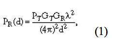
Where PT is the transmit power; PR (d) is the received power and a function of the distance d between the transmitter and the receiver; GT is the transmitter antenna gain; GR is the receiver antenna gain; d is the distance between the transmitter and receiver, in units Is metric; λ is the wavelength, and the unit is also metric.
The Friis free space equation shows that the received power decreases with the square of the distance between the transmitter and the receiver; in other words, the received power will decrease at a rate of 20 dB / decade as the distance increases.
Path loss is very important to estimate the wireless transmission distance. It is equal to the difference between the transmitted power and the received power (in decibels) and represents the degree of signal attenuation. It can be derived from equation (1) that the path loss is equal to the transmitted power divided by the received power, and equation (2) defines the path loss as:
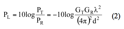
Where PL is the path loss. Assuming that both the transmitting and receiving antennas are unity, equation (2) can be simplified to:
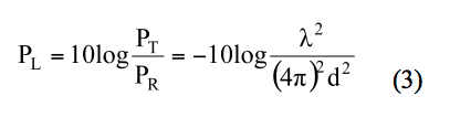
This equation can also be expressed in the following useful form:
PL = 20log10 (fMHz) + 20log10 (d) – 28 (4)
Or
PR = PT – PL (5)
Where d is the distance in meters.
Only when the value of d is in the far field of the transmitting antenna, the Friis free space formula can estimate the received power intensity. The far field of the transmitting antenna is also called the Fraunhofer area, which refers to the area beyond the antenna's far field distance dF. The dF of the antenna is equal to 2D2 / λ, where D is the largest physical linear dimension of the antenna; in addition, dF must also be greater than D, and it must be in the far field area. This path loss formula is only applicable to the ideal system where the transmitter and receiver are in line of sight of each other, and only for preliminary estimation.
The propagation model regards the close-in distance d0 as the received power reference point, and the designer must use the received power PR (d0) of this reference point to calculate the received power when the distance is greater than d0. Designers can use equations 1 and 4 to predict PR (d0), or measure the received power at many points near the transmitter, and then use their average value as PR (d0). When the designer selects the short-range reference point, he must determine that the far-field area is beyond the short-range distance.
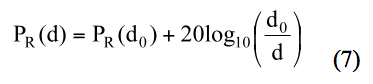
Designers can use this information and the following formula to calculate the received power at any distance:
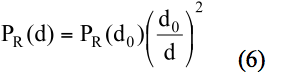
For an actual system operating in the 1-2 GHz range, the reference distance for the indoor environment is 1 meter, and the outdoor environment is 100 meters.
The commonly used unit of RF power intensity is milliwatt decibel or watt decibel, not absolute power intensity. Therefore, equation (6) can be expressed as:
The following example illustrates these concepts. Assuming a transmit frequency of 900 MHz, a transmit power of 6.3 mW (8 dBm), and using unity-gain transmit and receive antennas, the receive power at an outdoor line of sight of 1200 meters can be calculated as follows: the reference distance for the outdoor environment is 100 meters, 900 MHz The wavelength of the signal is 0.33 meters, so the received power at 100 meters can be calculated using the value of equation (1) as follows:
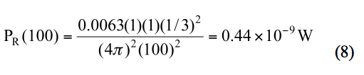
To calculate the milliwatt decibel power value, the power must be expressed as the following milliwatt value:
PR (100) = 0.44 × 10⁻⁶mW. (9)
This can be obtained:
PR (100) = 10log (0.44 × 10⁻⁶mW) = -63.6dBm. (10)
Using equation (7), the received power at 1200 meters can be obtained as:
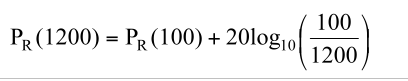 (11)
(11) as well as
PR (1200) = -63.6dBm – 21.58dB = -85dBm. (12)
You can also use equation (5) to verify that the received power is this value.
Therefore, in an ideal environment with no obstacles and line of sight, when the transmit power is 8 dBm, the received power at a distance of 1200 meters is about -85 dBm. Of course, the received power in the actual environment will be lower than the ideal value, because there may be obstacles between the target point and the transmitter, or simply out of sight. It is known from the previous example that the path loss is PT – PR, so it is equal to 8dBm – (-85dBm) = 93dB.
Actual path loss formula
Any practical wireless sensor system must know its maximum reliable transmission distance. The transmission distance of this wireless system is directly determined by the link budget parameters:
LB = PT + GT + GR – RS (13)
Where LB is the link budget in decibels, PT is the transmit power in milliwatts or watts decibels, GT is the transmitter antenna gain in decibels, GR is the receiver antenna gain in decibels, and RS is the receiver Sensitivity represents the minimum RF signal that the system can detect and provide an appropriate signal-to-clutter ratio. The receiver sensitivity is shown in Equation 14:
S = -174dBm / Hz + NF + 10logB + SNRMIN (14)
Among them, -174dBm / Hz is the thermal noise reference, NF is the total noise figure of the receiver in decibels, B is the total bandwidth of the receiver, and SNRMIN is the minimum signal-to-noise ratio. If the total path loss between the transmitter and the target receiver is greater than the link budget, data will be lost and communication will not be possible. Therefore, designers must accurately analyze the path loss characteristics when developing the final system and compare it with the link budget to obtain a preliminary distance estimate.
Indoor channel path loss
The indoor radio channel is different from the outdoor channel, because the indoor channel has a shorter transmission distance and the channel loss has a large change, so the received signal strength changes greatly. But for fixed wireless devices, this part is negligible. The layout, type and building materials of the building will have a great influence on indoor signal propagation. The researchers divided indoor channels into two types, one with line of sight and the other with channels blocked to varying degrees (Reference 1). The internal and external structures of a building may contain many different compartments and obstacles, depending on whether the building is in a home or office environment. The compartments of the building structure are fixed compartments, the movable compartments can move around, and the top of the compartments will not touch the ceiling. Families usually use wooden partitions, while office buildings use reinforced concrete between floors and mobile partitions.
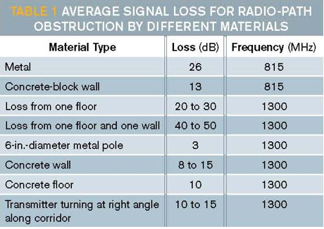
Buildings have many different compartments, and their physical and electrical characteristics are also very different. It is difficult to rely on a general model to analyze indoor channels. However, after extensive research, the industry has tabulated the signal loss of commonly used materials (Table 1).
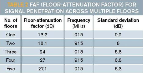
The floor attenuation factor represents the isolation loss between floors (Table 2).
Equation (15) is the actual path loss model of the indoor channel obtained by using the log distance path loss model:
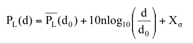 (15)
(15) Where X is a zero-average Gaussian random variable in decibels and σ is the standard deviation. If it is a fixed device, the effect of Xσ can be ignored. Use equation (4) to calculate the path loss value at a distance of 1 meter, and then substitute the result into equation 15 to get:
PL (d) = 20log10 (fMHz) + 10nlog10 (d) – 28 + Xσ (16)
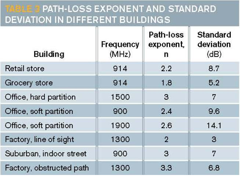
The value of n will not change much with the frequency, but will be affected by the surrounding environment and the type of building (Table 3).
The propagation model in the building contains the influence of the building type and obstacles. This model is not only flexible, but also reduces the standard deviation between the measured and predicted path loss to about 4dB, which is better than 13dB when using the log-distance model only. Equation 17 represents the attenuation factor model:
PL (d) = 20log10 (fMHz) + 10nSFlog10 (d) – 28 + FAF (17)
Among them, nSF represents the path loss index when measuring on the same floor, and FAF is the floor attenuation factor (Table 3). The designer can determine the floor attenuation factor according to Table 2. The following example demonstrates how to use the aforementioned table and equations. It uses the following formula to calculate the path loss of 915MHz and 2.4GHz signals in an outdoor open environment at a distance of 1200 meters:
20log10 (fMHz) + 20log10 (d) – 28 (18)
The path loss of 915MHz can be obtained from the above formula:
915MHz = 20log10 (915) + 20log10 (1200) – 28 = 92.8 dB (19)
The path loss of 2400MHz is:
2400MHz = 20log10 (2400) + 20log10 (1200) – 28 = 101.2 dB (20)
The higher the frequency of the transmitted signal, the greater the path loss, which will shorten the wireless transmission distance of high-frequency signals. For example, in an open outdoor environment, 2.4GHz wireless devices have approximately 8.4dB more path loss than 915MHz devices.
Another example is to take the office environment of fixed compartments on the same floor and three floors as the object, and use the data in Table 2 to calculate the path loss of 915MHz and 2.4GHz signals at a distance of 100 meters. It can be seen from Table 3 that the average path loss on the same floor is 3dBm, and substitute this value of n = 3 into the following formula:
20log10 (fMHz) + 10log10 (d) – 28 + Xσ (21)
The path loss at 915MHz can be obtained as:
915MHz = 20log10 (915) + 10 (3) log (100) – 28 + Xσ = 91.2dB (22)
Where σ = 7dB. The path loss of 2400MHz is:
2400MHz = 20log10 (2400) + 10 (3) log (100) – 28 + Xσ = 99.6dB (23)
Where σ = 14dB.
From Table 2, the floor attenuation factor of the three-story building can be calculated to be about 24dB, and the standard deviation is 5.6dB. Put this information into the following formula:
20log10 (fMHz) + 10log10 (d) – 28 + Xσ (24)
The path loss at 915MHz can be obtained as:
915MHz = 20log10 (915) + 10 (3) log10 (100) – 28 + 24 = 115.2dB (25)
Where σ = 5.6dB. The path loss of 2400MHz is:
2400MHz = 20log10 (2400) + 10 (3) log10 (100) – 28 + 24 = 123.6dB, (26)
Where σ = 5.9dB.
The third example assumes that the system uses unity-gain transmit and receive antennas, a transmit power of 8 dBm, and a receiver sensitivity of -100 dBm, and then estimates the transmission distance of the 915 MHz signal in the first two examples. Note that the system link budget at this time is 8 – (-100) = 108dB.
To illustrate the standard deviation in the path loss formula, it is best to reserve a margin of around 10dB for the link budget. This means that the available link budget is 98dB, which exceeds the 92.8dB path loss of the first example; therefore, designers can view the system's outdoor transmission distance as 1200 meters. In an indoor environment, the path loss is 91.2dB, and the available link budget when the 10dB margin is reserved is about 98dB, which also exceeds the path loss. Therefore, designers can regard the indoor transmission distance of the system as 100 meters.
Sijee Fiber optic adaptors are part of passive components for FTTH ODN connectivity, Sijee Fiber optic adaptors are used to join two fiber optic patch cables together for realizing the transition between different interfaces and they are available for use with either single-mode or multimode Fiber Optic Patch Cord. Sijee Fiber optic adaptors can offer superior low loss performance with very high repeatability.
Sijee offers different types of fiber adaptors comply with ITU standard, main products including Fiber Mating Sleeve Adaptor, Fiber Hybrid Adaptor, Fiber Bare Fiber Adaptor , Fiber Mechanical Attenuator, Field Assembly Optical Connector (FAOC), Splice-On Connector, Semi-finished Fiber Connector, etc.
Optical Fiber Couplers,Optical Fiber Adapter,Fiber Optic Adapter, Fiber Optic Flange are available.
Features:
1. Compliant with: IEC, JIS, Telcordia
2. Convenience and ease of handling
3. Optical performance 100% factory tested
4. Flange or threaded mounting type
5. Ceramic/Zirconia or phosphorous bronze sleeves
6. Good changeability and repeatability
Applications:
1. Telecommunication networks
2. FTTX, FTTH
3. LAN, WAN, CATV networks
4. Fiber communications, Data communication networks and processing, Industrial, Mechanical and Military.
5. Active device termination


Fiber Adaptor
Optical Fiber Couplers,Optical Fiber Adapter,Fiber Optic Adapter,Fiber Optic Flange
Sijee Optical Communication Technology Co.,Ltd , https://www.sijee-optical.com