Abstract: Today's low-power microcontrollers (μC) have also begun to integrate peripheral functions that originally existed only in large microprocessors, ASICs, and DSPs, making it possible for us to implement complex arithmetic operations with low power consumption. This article discusses a Fast Fourier Transform (FFT) application and implements the application on a low-power μC with a single-cycle hardware multiplier.
This FFT application calculates the spectrum of an input voltage (VIN in Figure 1) in real time. To accomplish this task, a piece of analog-to-digital converter (ADC) is used to sample VIN, and the obtained sample is transferred to µC. Then, µC performs a 256-point FFT on these samples to obtain the frequency spectrum of the input voltage. To facilitate detection, µC transmits the calculated spectrum data to the PC, which displays it in real time.
Figure 1. Using the FFT application to calculate the frequency spectrum of the input voltage.
The firmware for this FFT application is written in C for a 16-bit, low-power µC in the MAXQ2000 series. Interested readers can download (ZIP, 2.4kb) the firmware and circuit schematic of the project. Background To determine the frequency spectrum of input signal samples, we need to perform discrete Fourier transform (DFT) on these input samples. The definition of DFT is as follows:
Where N is the number of samples, X (k) is the spectrum, and x (n) is a set of input samples. Using Euler's equation to expand the summation operator, and to separate the real and imaginary parts of the input samples and the spectrum, the following equation is obtained:


In Equations 2 and 3, the second term in the summator disappears because the input samples are all real numbers. Assuming we have N samples, directly calculating Equations 2 and 3 requires 2N² multiplications and 2N (N-1) additions. In this way, our 256-point input sampling DFT will require 131,072 multiplications and 130,560 additions. Let's turn our attention to FFT!
There are multiple FFT algorithms available. This application uses the ordinary radix-2 algorithm and continues to decompose the DFT into two smaller DFTs. For this, N must be an exponent of 2. The steps of this radix-2 FFT algorithm can be summarized as the butterfly operation shown in Figure 2. Observing these butterfly operations, we can find that the radix-2 algorithm only requires (N / 2) log2 (N) multiplications and Nlog2 (N) additions. The parameter WN used in Figure 2 is the so-called "rotation factor", which can be calculated in advance before executing the algorithm.
Figure 2. Using butterfly operation to achieve FFT with N = 8.
In Figure 2, the input of the FFT is shown as a special arrangement sequence, which is obtained by inverting the binary digits of the original sequence index number. Therefore, when we execute the radix-2 FFT algorithm for N = 8 samples, we need to convert the original sequence of the input data:
0 (000b), 1 (001b), 2 (010b), 3 (011b), 4 (100b), 5 (101b), 6 (110b), 7 (111b)
Rearranged to:
0 (000b), 4, (100b), 2 (010b), 6 (110b), 1 (001b), 5 (101), 3 (011), 7 (111)
The FFT output is arranged in the correct order. Figure 2 also shows that the result of each individual butterfly operation is the only data required for the next FFT operation. Since the calculation process can be carried out "in place", the new value can replace the old value, so that only 2N variables are needed to calculate the FFT of N samples (because each data includes both real and imaginary parts).
After the FFT is completed, the result is in complex form. Equations 4 and 5 convert the result to polar coordinates and express it as:


Many optimization methods can be found in the literature on DSP, which can make the above DFT / FFT algorithm smaller or faster. One of the most important optimization methods (probably also the easiest to implement) stems from the fact that as a real signal, its DFT amplitude is symmetric with respect to X (N / 2), so:

Writing FFT code is never easy. Some limitations of low-power µC further complicate this task.
Memory: Our chosen µC has 2kB of RAM. It is known that the algorithm needs to use 2N 16-bit variables to store FFT data, so that our µC can perform FFT with N up to 512. However, some RAM is used in other parts of the firmware. Therefore, in this project, we limit N to 256. If a 16-bit variable is used to represent the real and imaginary parts of each value, a total of 1024 bytes of RAM are required for FFT data.
Speed: Despite its high MIPS / mA performance, low-power µC still requires some optimization to keep the number of instructions to run the FFT as small as possible. Fortunately, the C compiler used in this application (IAR's Embedded Workbench for MAXQ, see) can provide multiple levels of optimization and settings. Efficient use of hardware multipliers can optimize code to an acceptable level.
No floating-point capability: The selected µC does not have floating-point capability (low-power products generally do not have floating-point capability). Therefore, all operations must use fixed-point algorithms. To represent decimals, the firmware uses signed Q8.7 notation. In this way, it is assumed in the firmware that the 0th to 6th digits represent the decimal part, the 7th to 14th digits represent the integer part, and the 15th digit represents the sign bit (two's complement). This arrangement has no effect on addition and subtraction, but When doing multiplications, care must be taken to align the data according to the Q8.7 format.
The data representation chosen must also be adapted to the maximum value that the FFT algorithm may encounter while providing sufficient accuracy. For example, our ADC can provide signed 8-bit samples, expressed in two's complement. If the input is a DC voltage of maximum amplitude (127 for signed 8-bit samples), then its energy spectrum is all contained in X (0), which is represented by Q8.7 as 32512. This value can be represented by a single signed 16-bit data. Firmware The following section discusses the firmware implementation of radix-2 FFT on low-power µC. The signal samples are stored in the x_n_re array after being read out by the ADC. This array represents the real part of x (n). The imaginary part is stored in the x_n_im array and initialized to zero before starting the FFT. After the FFT is completed, the calculation result replaces the original sampled data and is stored in x_n_re and x_n_im. The acquisition sampling FFT algorithm assumes that the sampling is obtained at a fixed sampling frequency. If you are not careful when acquiring samples for the FFT, there will be some problems. For example, the jitter of the sampling interval will introduce errors into the FFT result, and every effort should be made to reduce it.
Decision sentences in the ADC sampling cycle will cause jitter in the sampling interval. For example, our system reads signed 8-bit samples from the ADC and stores them in a set of 16-bit variables. Two pseudo-code algorithms are given in the following program listing 1 to perform this ADC read-store function. The method given in Algorithm 1 will cause jitter in the sampling interval because negative sampling requires more time to read and store than positive sampling.
Listing 1. Two ADC sampling pseudocode algorithms. The second algorithm avoids the first problem-sampling interval jitter. // ALGORITHM 1: INCONSISTENT SAMPLING FREQUENCY-BAD! // sample [] is an array of 16-bit variables for i = 0 to (N-1) begin doADCSampleConversion () // Instruct ADC to sample Vin sample [i] = read8BitSampleFromADC () // Read 8-bit sample from ADC if (sample [i] & 0x0080) // If the 8-bit sample was negaTIve sample [i] = sample [i] + 0xFF00 // Make the 16-bit word negaTIve end // ALGORITHM 2: FIXED SAMPLING FREQUENCY-GOOD! // sample [] is an array of 16-bit variables for i = 0 to (N-1) begin doADCSampleConversion () // Instruct ADC to sample Vin sample [i ] = read8BitSampleFromADC () // Read 8-bit sample from ADC end for i = 0 to (N-1) begin if (sample [i] & 0x0080) // If the 8-bit sample was negaTIve sample [i] = sample [i] + 0xFF00 // Make the 16-bit word negaTIve end Trigonometric function table This FFT algorithm obtains the sine or cosine function value by looking up the table (LUT) instead of calculating. Listing 2 shows the declaration of sine and cosine LUT. The actual firmware notes contain the source code that automatically generates these LUTs, which can be called by the program. Both LUTs contain an N / 2 component because the index number of the rotation factor varies from 0 to N / 2-1 (see Figure 2).
Listing 2. Sine and cosine function LUT. const int cosLUT [N / 2] = {+ 128, + 127, + 127, ..., -127, -127, -127}; const int sinLUT [N / 2] = {+0, + 3, + 6, ..., +9, +6, +3}; The arrays in these LUTs are declared as const, forcing the compiler to store them in code space instead of data space. Since the LUT values ​​must be expressed in Q8.7, they are obtained by multiplying the actual values ​​of sine and cosine by 27. Bit reversal Bit reversal sorting (N known) can be written at run time by calculation, table lookup, or directly using unrolled loops. All of these methods require a compromise between the size and running speed of the source code. This FFT application uses unrolled loops to perform bit inversion. Its source code is long, but it runs fast. Listing 3 shows the implementation of this unrolled loop. The comments of this application firmware include the source code for the program to automatically generate and expand the loop.
Listing 3. An unrolled loop for implementing bit reversal of N = 256. i = x_n_re [1]; x_n_re [1] = x_n_re [128]; x_n_re [128] = i; i = x_n_re [2]; x_n_re [2] = x_n_re [64]; x_n_re [64] = i; i = x_n_re [3]; x_n_re [3] = x_n_re [192]; x_n_re [192] = i; i = x_n_re [4]; x_n_re [4] = x_n_re [32]; x_n_re [32] = i; ... i = x_n_re [207]; x_n_re [207] = x_n_re [243]; x_n_re [243] = i; i = x_n_re [215]; x_n_re [215] = x_n_re [235]; x_n_re [235] = i; i = x_n_re [223]; x_n_re [223] = x_n_re [251]; x_n_re [251] = i; i = x_n_re [239]; x_n_re [239] = x_n_re [247]; x_n_re [247] = i; Radix-2 FFT algorithm After the samples are reordered according to the bit reversal method, the FFT operation can be performed. The firmware of this radix-2 FFT application performs the butterfly operation shown in Figure 2 through three main loops. The outer loop counts log2 (N) FFT operations. The inner loop performs the butterfly operation of each stage.
The core part of the FFT algorithm is a small block of code that performs butterfly operations. Listing 4 shows this piece of code. Unfortunately, it is the only "non-portable" firmware in this application. Macros MUL_1 and MUL_2 use µC hardware multipliers to perform single instruction cycle multiplication. The contents of these macros are dedicated to the MAXQ2000, and can all be seen in the actual firmware.
Listing 4. Butterfly operation written in C. / * (1) Macro MUL_1 (A, B, C): C = A * B (result in Q8.7) * / / * (2) Macro MUL_2 (A, C): C = A * last_B (result in Q8.7) * / MUL_1 (cosLUT [tf], x_n_re [b], resultMulReCos); MUL_2 (sinLUT [tf], resultMulReSin); MUL_1 (cosLUT [tf], x_n_im [b], resultMulImCos); MUL_2 (sinLUT [ tf], resultMulImSin); x_n_re [b] = x_n_re [a] -resultMulReCos + resultMulImSin; x_n_im [b] = x_n_im [a] -resultMulReSin-resultMulImCos; x_n_re [a] = Re_m_res_MulImRes [M] a] = x_n_im [a] + resultMulReSin + resultMulImCos; The conversion of complex polar coordinates In order to facilitate the determination of the amplitude of the VIN spectrum, we need to convert the complex form of X (k) to polar coordinates. The firmware that implements this conversion is shown in Listing 5. The amplitude value replaces the original FFT result because the firmware no longer needs the data.
Listing 5. FFT results are converted from complex to polar form. const unsigned char magnLUT [16] [16] = {{0x00,0x10,0x20, ..., 0xd0,0xe0,0xf0}, {0x10,0x16,0x23, ..., 0xd0,0xe0,0xf0}, .. . {0xe0,0xe0,0xe2, ..., 0xff, 0xff, 0xff}, {0xf0,0xf0,0xf2, ..., 0xff, 0xff, 0xff}}; ... / * Compute x_n_re = abs (x_n_re) and x_n_im = abs (x_n_im) * / ... x_n_re [0] = magnLUT [x_n_re [0] >> 11] [0]; for (i = 1; i > 11] [x_n_im [i] >> 11]; x_n_re [N_DIV_2] = magnLUT [x_n_re [N_DIV_2] >> 11] [0]; The spectrum amplitude is not calculated according to Equation 4, but through a two-dimensional LUT look-up table get. The first index is the higher 4 bits (MSB) of the real part of the spectrum, and the second index is the higher 4 bits of the imaginary part of the spectrum. To get these data, the signed 16-bit data can be shifted right 11 times. Before obtaining the index numbers from the real and imaginary parts of the spectrum, they need to be converted to absolute values ​​first. Therefore, the sign bit is zero.
From Equation 6, we already know that the amplitude of the spectrum is symmetric about X (N / 2), so we only need to convert the first (N / 2) + 1 spectrum data into polar coordinates. Also, we can see that for real input samples, the imaginary parts of X (0) and X (N / 2) are always zero. Therefore, the amplitudes of the two spectral lines are calculated separately. The actual firmware of this project contains the source code for automatically generating the LUT, which can be called by the program to calculate the amplitude of X (k). Hamming or Hann window This project firmware also includes LUT (Q8.7 format) with Hamming or Hann window added to the input samples. The windowing function can effectively reduce the spectral leakage caused by the rounding operation of time domain sampling x (n). Hamming and Hann window functions are shown in Equations 7 and 8, respectively.


Listing 6 shows the code to implement these functions. Similarly, the actual firmware of the project contains the source code for automatically generating these LUTs, which can be called by the program to implement these window functions.
Listing 6. LUT used to implement Hamming and Hann window functions const char hammingLUT [N] = {+10, +10, +10, ..., + 10, +10, +10}; const char hannLUT [N] = {+0, +0, +0, .. ., +0, +0, +0}; ... ... for (i = 0; i <256; i ++) {#ifdef WINDOWING_HAMMING MUL_1 (x_n_re [i], hammingLUT [i], x_n_re [i] ); // x (n) * = hamming (n); #endif #ifdef WINDOWING_HANN MUL_1 (x_n_re [i], hannLUT [i]), x_n_re [i]); // x (n) * = hann (n ); #endif} Test results To test the performance of the FFT application, the firmware uploads the X (k) amplitude to the PC via the µC UART port. The specially written FFT Graph software (provided with the project firmware) is used to read these amplitudes from the PC serial port and display the spectrum in real time in a graphical manner. Figure 3 shows the results displayed by FFT Graph after sampling and processing four different input signals at 200ksps in µC: 4.3V DC signal 50kHz sinusoidal signal 70kHz sinusoidal signal 6.25kHz square wave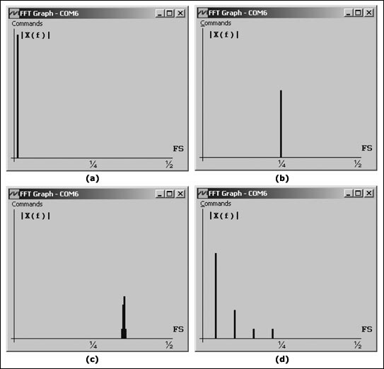
Figure 3. FFT Graph software shows the spectrum calculated from low-power µC.
This FFT application calculates the spectrum of an input voltage (VIN in Figure 1) in real time. To accomplish this task, a piece of analog-to-digital converter (ADC) is used to sample VIN, and the obtained sample is transferred to µC. Then, µC performs a 256-point FFT on these samples to obtain the frequency spectrum of the input voltage. To facilitate detection, µC transmits the calculated spectrum data to the PC, which displays it in real time.
Figure 1. Using the FFT application to calculate the frequency spectrum of the input voltage.
The firmware for this FFT application is written in C for a 16-bit, low-power µC in the MAXQ2000 series. Interested readers can download (ZIP, 2.4kb) the firmware and circuit schematic of the project. Background To determine the frequency spectrum of input signal samples, we need to perform discrete Fourier transform (DFT) on these input samples. The definition of DFT is as follows:
Where N is the number of samples, X (k) is the spectrum, and x (n) is a set of input samples. Using Euler's equation to expand the summation operator, and to separate the real and imaginary parts of the input samples and the spectrum, the following equation is obtained:
In Equations 2 and 3, the second term in the summator disappears because the input samples are all real numbers. Assuming we have N samples, directly calculating Equations 2 and 3 requires 2N² multiplications and 2N (N-1) additions. In this way, our 256-point input sampling DFT will require 131,072 multiplications and 130,560 additions. Let's turn our attention to FFT!
There are multiple FFT algorithms available. This application uses the ordinary radix-2 algorithm and continues to decompose the DFT into two smaller DFTs. For this, N must be an exponent of 2. The steps of this radix-2 FFT algorithm can be summarized as the butterfly operation shown in Figure 2. Observing these butterfly operations, we can find that the radix-2 algorithm only requires (N / 2) log2 (N) multiplications and Nlog2 (N) additions. The parameter WN used in Figure 2 is the so-called "rotation factor", which can be calculated in advance before executing the algorithm.
Figure 2. Using butterfly operation to achieve FFT with N = 8.
In Figure 2, the input of the FFT is shown as a special arrangement sequence, which is obtained by inverting the binary digits of the original sequence index number. Therefore, when we execute the radix-2 FFT algorithm for N = 8 samples, we need to convert the original sequence of the input data:
0 (000b), 1 (001b), 2 (010b), 3 (011b), 4 (100b), 5 (101b), 6 (110b), 7 (111b)
Rearranged to:
0 (000b), 4, (100b), 2 (010b), 6 (110b), 1 (001b), 5 (101), 3 (011), 7 (111)
The FFT output is arranged in the correct order. Figure 2 also shows that the result of each individual butterfly operation is the only data required for the next FFT operation. Since the calculation process can be carried out "in place", the new value can replace the old value, so that only 2N variables are needed to calculate the FFT of N samples (because each data includes both real and imaginary parts).
After the FFT is completed, the result is in complex form. Equations 4 and 5 convert the result to polar coordinates and express it as:
Many optimization methods can be found in the literature on DSP, which can make the above DFT / FFT algorithm smaller or faster. One of the most important optimization methods (probably also the easiest to implement) stems from the fact that as a real signal, its DFT amplitude is symmetric with respect to X (N / 2), so:
Writing FFT code is never easy. Some limitations of low-power µC further complicate this task.
Memory: Our chosen µC has 2kB of RAM. It is known that the algorithm needs to use 2N 16-bit variables to store FFT data, so that our µC can perform FFT with N up to 512. However, some RAM is used in other parts of the firmware. Therefore, in this project, we limit N to 256. If a 16-bit variable is used to represent the real and imaginary parts of each value, a total of 1024 bytes of RAM are required for FFT data.
Speed: Despite its high MIPS / mA performance, low-power µC still requires some optimization to keep the number of instructions to run the FFT as small as possible. Fortunately, the C compiler used in this application (IAR's Embedded Workbench for MAXQ, see) can provide multiple levels of optimization and settings. Efficient use of hardware multipliers can optimize code to an acceptable level.
No floating-point capability: The selected µC does not have floating-point capability (low-power products generally do not have floating-point capability). Therefore, all operations must use fixed-point algorithms. To represent decimals, the firmware uses signed Q8.7 notation. In this way, it is assumed in the firmware that the 0th to 6th digits represent the decimal part, the 7th to 14th digits represent the integer part, and the 15th digit represents the sign bit (two's complement). This arrangement has no effect on addition and subtraction, but When doing multiplications, care must be taken to align the data according to the Q8.7 format.
The data representation chosen must also be adapted to the maximum value that the FFT algorithm may encounter while providing sufficient accuracy. For example, our ADC can provide signed 8-bit samples, expressed in two's complement. If the input is a DC voltage of maximum amplitude (127 for signed 8-bit samples), then its energy spectrum is all contained in X (0), which is represented by Q8.7 as 32512. This value can be represented by a single signed 16-bit data. Firmware The following section discusses the firmware implementation of radix-2 FFT on low-power µC. The signal samples are stored in the x_n_re array after being read out by the ADC. This array represents the real part of x (n). The imaginary part is stored in the x_n_im array and initialized to zero before starting the FFT. After the FFT is completed, the calculation result replaces the original sampled data and is stored in x_n_re and x_n_im. The acquisition sampling FFT algorithm assumes that the sampling is obtained at a fixed sampling frequency. If you are not careful when acquiring samples for the FFT, there will be some problems. For example, the jitter of the sampling interval will introduce errors into the FFT result, and every effort should be made to reduce it.
Decision sentences in the ADC sampling cycle will cause jitter in the sampling interval. For example, our system reads signed 8-bit samples from the ADC and stores them in a set of 16-bit variables. Two pseudo-code algorithms are given in the following program listing 1 to perform this ADC read-store function. The method given in Algorithm 1 will cause jitter in the sampling interval because negative sampling requires more time to read and store than positive sampling.
Listing 1. Two ADC sampling pseudocode algorithms. The second algorithm avoids the first problem-sampling interval jitter. // ALGORITHM 1: INCONSISTENT SAMPLING FREQUENCY-BAD! // sample [] is an array of 16-bit variables for i = 0 to (N-1) begin doADCSampleConversion () // Instruct ADC to sample Vin sample [i] = read8BitSampleFromADC () // Read 8-bit sample from ADC if (sample [i] & 0x0080) // If the 8-bit sample was negaTIve sample [i] = sample [i] + 0xFF00 // Make the 16-bit word negaTIve end // ALGORITHM 2: FIXED SAMPLING FREQUENCY-GOOD! // sample [] is an array of 16-bit variables for i = 0 to (N-1) begin doADCSampleConversion () // Instruct ADC to sample Vin sample [i ] = read8BitSampleFromADC () // Read 8-bit sample from ADC end for i = 0 to (N-1) begin if (sample [i] & 0x0080) // If the 8-bit sample was negaTIve sample [i] = sample [i] + 0xFF00 // Make the 16-bit word negaTIve end Trigonometric function table This FFT algorithm obtains the sine or cosine function value by looking up the table (LUT) instead of calculating. Listing 2 shows the declaration of sine and cosine LUT. The actual firmware notes contain the source code that automatically generates these LUTs, which can be called by the program. Both LUTs contain an N / 2 component because the index number of the rotation factor varies from 0 to N / 2-1 (see Figure 2).
Listing 2. Sine and cosine function LUT. const int cosLUT [N / 2] = {+ 128, + 127, + 127, ..., -127, -127, -127}; const int sinLUT [N / 2] = {+0, + 3, + 6, ..., +9, +6, +3}; The arrays in these LUTs are declared as const, forcing the compiler to store them in code space instead of data space. Since the LUT values ​​must be expressed in Q8.7, they are obtained by multiplying the actual values ​​of sine and cosine by 27. Bit reversal Bit reversal sorting (N known) can be written at run time by calculation, table lookup, or directly using unrolled loops. All of these methods require a compromise between the size and running speed of the source code. This FFT application uses unrolled loops to perform bit inversion. Its source code is long, but it runs fast. Listing 3 shows the implementation of this unrolled loop. The comments of this application firmware include the source code for the program to automatically generate and expand the loop.
Listing 3. An unrolled loop for implementing bit reversal of N = 256. i = x_n_re [1]; x_n_re [1] = x_n_re [128]; x_n_re [128] = i; i = x_n_re [2]; x_n_re [2] = x_n_re [64]; x_n_re [64] = i; i = x_n_re [3]; x_n_re [3] = x_n_re [192]; x_n_re [192] = i; i = x_n_re [4]; x_n_re [4] = x_n_re [32]; x_n_re [32] = i; ... i = x_n_re [207]; x_n_re [207] = x_n_re [243]; x_n_re [243] = i; i = x_n_re [215]; x_n_re [215] = x_n_re [235]; x_n_re [235] = i; i = x_n_re [223]; x_n_re [223] = x_n_re [251]; x_n_re [251] = i; i = x_n_re [239]; x_n_re [239] = x_n_re [247]; x_n_re [247] = i; Radix-2 FFT algorithm After the samples are reordered according to the bit reversal method, the FFT operation can be performed. The firmware of this radix-2 FFT application performs the butterfly operation shown in Figure 2 through three main loops. The outer loop counts log2 (N) FFT operations. The inner loop performs the butterfly operation of each stage.
The core part of the FFT algorithm is a small block of code that performs butterfly operations. Listing 4 shows this piece of code. Unfortunately, it is the only "non-portable" firmware in this application. Macros MUL_1 and MUL_2 use µC hardware multipliers to perform single instruction cycle multiplication. The contents of these macros are dedicated to the MAXQ2000, and can all be seen in the actual firmware.
Listing 4. Butterfly operation written in C. / * (1) Macro MUL_1 (A, B, C): C = A * B (result in Q8.7) * / / * (2) Macro MUL_2 (A, C): C = A * last_B (result in Q8.7) * / MUL_1 (cosLUT [tf], x_n_re [b], resultMulReCos); MUL_2 (sinLUT [tf], resultMulReSin); MUL_1 (cosLUT [tf], x_n_im [b], resultMulImCos); MUL_2 (sinLUT [ tf], resultMulImSin); x_n_re [b] = x_n_re [a] -resultMulReCos + resultMulImSin; x_n_im [b] = x_n_im [a] -resultMulReSin-resultMulImCos; x_n_re [a] = Re_m_res_MulImRes [M] a] = x_n_im [a] + resultMulReSin + resultMulImCos; The conversion of complex polar coordinates In order to facilitate the determination of the amplitude of the VIN spectrum, we need to convert the complex form of X (k) to polar coordinates. The firmware that implements this conversion is shown in Listing 5. The amplitude value replaces the original FFT result because the firmware no longer needs the data.
Listing 5. FFT results are converted from complex to polar form. const unsigned char magnLUT [16] [16] = {{0x00,0x10,0x20, ..., 0xd0,0xe0,0xf0}, {0x10,0x16,0x23, ..., 0xd0,0xe0,0xf0}, .. . {0xe0,0xe0,0xe2, ..., 0xff, 0xff, 0xff}, {0xf0,0xf0,0xf2, ..., 0xff, 0xff, 0xff}}; ... / * Compute x_n_re = abs (x_n_re) and x_n_im = abs (x_n_im) * / ... x_n_re [0] = magnLUT [x_n_re [0] >> 11] [0]; for (i = 1; i
From Equation 6, we already know that the amplitude of the spectrum is symmetric about X (N / 2), so we only need to convert the first (N / 2) + 1 spectrum data into polar coordinates. Also, we can see that for real input samples, the imaginary parts of X (0) and X (N / 2) are always zero. Therefore, the amplitudes of the two spectral lines are calculated separately. The actual firmware of this project contains the source code for automatically generating the LUT, which can be called by the program to calculate the amplitude of X (k). Hamming or Hann window This project firmware also includes LUT (Q8.7 format) with Hamming or Hann window added to the input samples. The windowing function can effectively reduce the spectral leakage caused by the rounding operation of time domain sampling x (n). Hamming and Hann window functions are shown in Equations 7 and 8, respectively.
Listing 6 shows the code to implement these functions. Similarly, the actual firmware of the project contains the source code for automatically generating these LUTs, which can be called by the program to implement these window functions.
Listing 6. LUT used to implement Hamming and Hann window functions const char hammingLUT [N] = {+10, +10, +10, ..., + 10, +10, +10}; const char hannLUT [N] = {+0, +0, +0, .. ., +0, +0, +0}; ... ... for (i = 0; i <256; i ++) {#ifdef WINDOWING_HAMMING MUL_1 (x_n_re [i], hammingLUT [i], x_n_re [i] ); // x (n) * = hamming (n); #endif #ifdef WINDOWING_HANN MUL_1 (x_n_re [i], hannLUT [i]), x_n_re [i]); // x (n) * = hann (n ); #endif} Test results To test the performance of the FFT application, the firmware uploads the X (k) amplitude to the PC via the µC UART port. The specially written FFT Graph software (provided with the project firmware) is used to read these amplitudes from the PC serial port and display the spectrum in real time in a graphical manner. Figure 3 shows the results displayed by FFT Graph after sampling and processing four different input signals at 200ksps in µC: 4.3V DC signal 50kHz sinusoidal signal 70kHz sinusoidal signal 6.25kHz square wave
Figure 3. FFT Graph software shows the spectrum calculated from low-power µC.
Wifi Control Vacuum Cleaner,Thinnest Robot Vacuum Cleaner ,Air Purifier Wifi Control,Low Noise Cleaner Robot
NingBo CaiNiao Intelligent Technology Co., LTD , https://www.intelligentnewbot.com